
How To: Inventory Run Out Date Based on Forecasts and Open Orders Excel
Figuring out when product inventory will run out seems like a simple enough task, but when you have thousands of items, changing forecasts, and multiple open orders with differing receipt dates, things start to get complicated quickly. This article will explain how to organize and display your data in a spreadsheet in order to efficiently identify your product run out dates.
Download the exercise file here, which I will be using to create the run out date information. It is divided into three sheets; Main Sheet, Open Orders, and Forecasts. These contain the baseline required information to find your run out dates. They are set up so you can update the forecasts and open order information to automatically update the run out dates.
The exercise file is set up to accommodate the next two open orders, but the same principles can be applied to an infinite number of open orders. It is also set up to start tracking information from the beginning of a year (January 1). The forecasts are set up using four weekly buckets, with the last bucket accounting for 2-3 additional days than the others.
There are many other options that can be added on if you are looking for in depth information about your products, this may include; lost sales during stock out periods, conditional flags for lead times that are greater than the run out date when no open orders are present, using the =TODAY() function to eliminate weekly updating of the buckets, will the next open order cover the potential back order or pent up demand, and doing all of these same calculations based on last X day sales averages in order to compare actual sales to forecasts.
With all of that said lets jump into how to actually do this.
Step by step
- Find run out dates for the available inventory; in cell E2 type {=IFERROR(INDEX($P$1:$BK$1,MATCH(TRUE,SUBTOTAL(9,OFFSET(P2:BK2,,,,COLUMN($P$1:$BK$1)-COLUMN(P2)+1))>+D2,0)),”None”)} note the CTRL+Shift+Enter used on this formula because of the array (the brackets ({}) at the beginning and end are not typed, they appear with the CTRL+Shift+Enter.
- Find the run out dates for the available inventory + open order #1 quantity; in cell J2 type {=IFERROR(INDEX($P$1:$BK$1,MATCH(TRUE,SUBTOTAL(9,OFFSET(P2:BK2,,,,COLUMN($P$1:$BK$1)-COLUMN(P2)+1))>+D2+H2,0)),”None”)} note the CTRL+Shift+Enter used on this formula because of the array (the brackets ({}) at the beginning and end are not typed, they appear with the CTRL+Shift+Enter.
- Find the run out dates for the available inventory + open order #1 and #2 quantity; in cell N2 type {=IFERROR(INDEX($P$1:$BK$1,MATCH(TRUE,SUBTOTAL(9,OFFSET(P2:BK2,,,,COLUMN($P$1:$BK$1)-COLUMN(P2)+1))>+D2+H2+L2,0)),”None”)} note the CTRL+Shift+Enter used on this formula because of the array (the brackets ({}) at the beginning and end are not typed, they appear with the CTRL+Shift+Enter.
- Find the stock out days till order #1; in cell K2 type =IFERROR(MAX(0,I2-E2),0)
- Find the stock out days till order #2; in cell O2 type =IFERROR(MAX(0,M2-J2),0)
- Find the run out date; in cell F2 type =IF(K2>0,E2,IF(AND(K2=0,O2>0),J2,N2))
- Find the stock out days; in cell G2 type =IF(SUM(H2,L2)=0,”No Open Orders”,IF(SUM(K2,O2)=0,”None”,IF(K2>0,K2,IF(AND(K2=0,O2>0),O2))))
- Use the information as you see fit
Definitions
Stock Out Days: the number of days the item will be unavailable. Stock out date till next receipt date.
No Open Orders: there are no open orders for this item, stock out days are indefinite.
None: all open orders are set to arrive before inventory run outs, but there are no additional open orders after the run out date.
Number: represents the number of days the item will be stocked out, beginning on the run out date and ending on the open order date that will replenish it.
Available inventory Run Out date: the date that available inventory runs out, if “None” then the forecasts will not consume the inventory to zero.
Run Out Date: the date that inventory levels will reach zero, this factors in available inventory, open order quantities and dates, and forecasts, if “None” then the forecasts will not consume the inventory to zero.
Explanations With Images
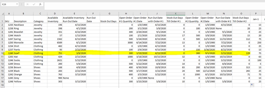
Download the exercise file here, It is divided into three sheets; Main Sheet, Open Orders, and Forecasts. The main sheet is where we will compiling all of the data and writing our formulas. Open orders contains information on open purchase orders including the item, quantity, and expected receipt date. Note that any given item can have 0-2 open orders, no open orders are indicated by blanks in the cells. The forecast sheet has the total monthly forecasts for each item broken out by month. The main sheet uses =VLOOKUP to draw in the data from the open orders and forecasts sheets. This allows for easy updating when information changes. Note that the forecast on the main sheet have been divided into four weeks for each month, with the last week of the month being slightly longer than the others. These are buckets with the date indicating the “week beginning.”
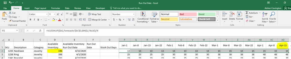
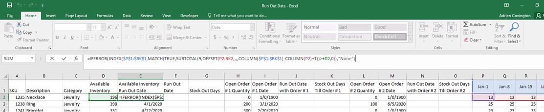
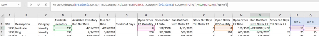
The first step is to find the run out dates for the currently available inventory. This tells you, “if no more units are received, when will the current inventory run out?” everything will be built off of this date. First let’s write the formula; in cell E2 type
{=IFERROR(INDEX($P$1:$BK$1,MATCH(TRUE,SUBTOTAL(9,OFFSET(P2:BK2,,,,COLUMN($P$1:$BK$1)-COLUMN(P2)+1))>+D2,0)),”None”)}
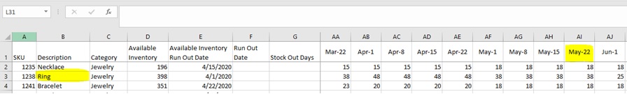
note the CTRL+Shift+Enter used on this formula because of the array (the brackets ({}) at the beginning and end are not typed, they appear with the CTRL+Shift+Enter. In Layman’s terms this is summing the forecasts for each consecutive week until it becomes larger than the current available inventory and then returns the weekly bucket in which it occurred. For our example of the necklace the available inventory is 196. So based on forecasts this inventory will run out the week of April 15, 2020. If you sum each weekly forecast amount starting in column P (Jan-1) and ending in column AD (Apr-15) it will equal 205, ending one week earlier on column AC (Apr-8) equals 190. Given this information you can expect to have 6 remaining units at the end of the Apr-8 week, which will run out the week of Apr-15.
I wont go into too much detail about how the formulas work, but here is an overview as these will used frequenlty thoughout the tuturial. It is primarily and INDEX + MATCH that uses an OFFSET for the column width based on the available inventory. If interested in learning more I suggest researching; INDEX + MATCH, OFFSET, and COLUMN formulas.
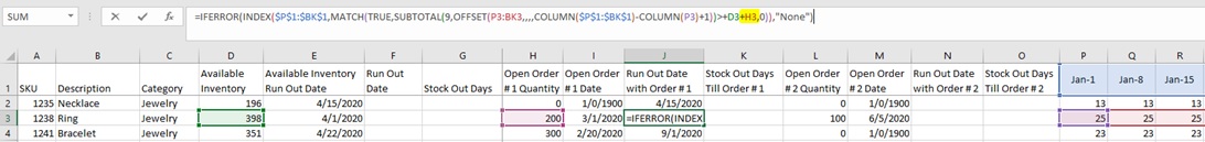
Next we will find the run out dates for the available inventory + open order #1 quantity. First let’s write the formula; in cell J2 type
{=IFERROR(INDEX($P$1:$BK$1,MATCH(TRUE,SUBTOTAL(9,OFFSET(P2:BK2,,,,COLUMN($P$1:$BK$1)-COLUMN(P2)+1))>+D2+H2,0)),”None”)}
note the CTRL+Shift+Enter used on this formula because of the array (the brackets ({}) at the beginning and end are not typed, they appear with the CTRL+Shift+Enter. Almost the exact same formula as in the first step except for this time we are adding in the open order #1 quantity. Essentially it is saying, “If the next order was here today and we added it to the currently available inventory, when would that inventory run out?” This is done by adding in the “+H3” at the end of the formula (highlighted below). Because the necklace on line 2 does not have any open orders, let’s take the ring on line three as an example; the available inventory of 398 units will run out the week of April 1. If we add the 200 additional units that are scheduled to arrive on the next order to the 398 we have currently, those 598 units will run out the week beginning May 8. At this point we are not concerned about the receipt date of the order, this will come into play later.

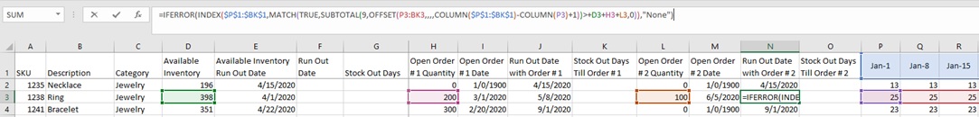
We will repeat the previous step, only this time adding in the second open order. In other words we will find the run out dates for the available inventory + open order #1 quantity + open order #2 quantity. First let’s write the formula; in cell N2 type
{=IFERROR(INDEX($P$1:$BK$1,MATCH(TRUE,SUBTOTAL(9,OFFSET(P2:BK2,,,,COLUMN($P$1:$BK$1)-COLUMN(P2)+1))>+D2+H2+L2,0)),”None”)}
note the CTRL+Shift+Enter used on this formula because of the array (the brackets ({}) at the beginning and end are not typed, they appear with the CTRL+Shift+Enter. Essentially it is saying, “If the next two orders were here today and we added it to the currently available inventory, when would that inventory run out?” This is done by adding in the “+L2” at the end of the previous formula (highlighted below). Let’s take the ring on line three as an example; the available inventory of 398 units will run out the week of April 1. If we add the 200 additional units that are scheduled to arrive on the next order and the 100 units on order #2 to the 398 we have currently, those 698 units will run out the week beginning May 22. At this point we are not concerned about the receipt date of the order, this will come into play later.
Now that we have all the run out dates we can start in on the stock out days. This is where the dates really start to come into play. If stock out days are showing then there is a difference between run out dates and one of the open orders dates. Let’s start with stock out dates till order #1. First let’s write the formula; in cell K2 type
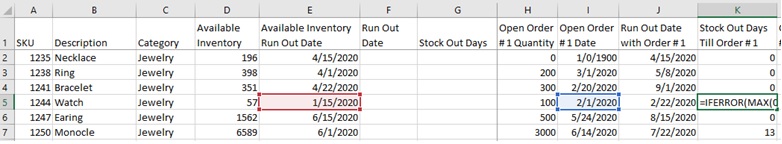
=IFERROR(MAX(0,I2-E2),0)
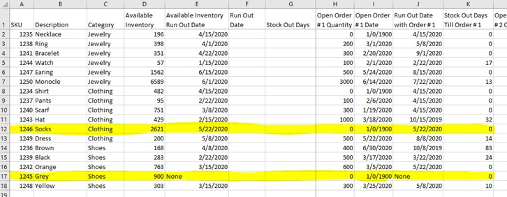
The first three rows of products don’t have a stock out period between available inventory and open order #1, but SKU 1244 Watch does. The 57 available units are set to run out the week of Jan 15, but the open order #1 won’t arrive until Feb 1. This results in 17 days of stock out where the product will be unavailable for purchase. Also worth noting is line 17 with the grey shoe, which does not have any stock out days because the available inventory will not be sold through for as far out as our forecasts go. Also notice line 12 where available inventory is running out May 22, and there are no open orders. This too will indicate no stock out days.
Stock out days till order #2 is done in much the same way as the previous step. First let’s write the formula; in cell O2 type
=IFERROR(MAX(0,M2-J2),0)
This accomplishes the same thing as the previous step except now we are getting the number of stock out days between order #1 and order #2. Taking a look at the Scarf on line 10 we can see that there are 139 days between the run out date with order #1 and the open order date for order #2.
Now that we have all the base information ready we can finally get the run out date for the product given open orders and forecasts. First let’s write the formula; in cell F2 type
=IF(K2>0,E2,IF(AND(K2=0,O2>0),J2,N2))
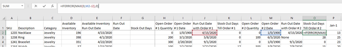
This formula is looking at the stock out days in columns K and O and if it finds a number greater than 0 then it return the run out date of the order # before it or the run out date of the available inventory. If both stock out days say 0 then it returns the run out date for order #2. So what it is saying is; if there is a projected stock out duration then that means an order is coming in too late thus the stock out date must occur before said open order. If we take a look at line 3 the Ring, you can see the run out date of 5/8/2020 this is due to no stock out days till order #1 (column K) and 28 stock out days till order #2 (column O). So it is saying that available inventory will run out on 4/1/2020 but order #1 arrives a month earlier on 3/1/2020 so those 200 units will arrive in time and then run out on 5/8/2020 and the order #2 won’t arrive till 6/5/2020.

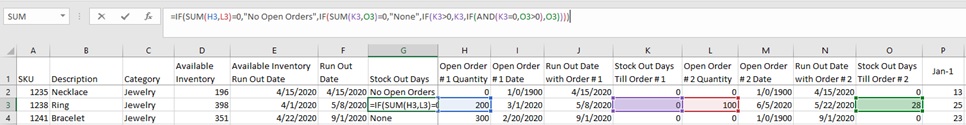
Finally to wrap it up we will get the stock out days to go with our run out date. First lets write the formula; in cell G2 type
=IF(SUM(H2,L2)=0,”No Open Orders”,IF(SUM(K2,O2)=0,”None”,IF(K2>0,K2,IF(AND(K2=0,O2>0),O2))))
What this is saying is; from the day the item will stock out (column F) how long till the next order comes in and inventory is replenished. If it returns “No Open Orders” then there are not any open orders and the item will stock out on the day indicated (available inventory run out date), if it says “None” then there are no more additional orders after the item is set to stock out but the open orders that do exist will arrive in time. If there is a number then that is the number of days that the item will be stocked out until an open order is received. All this formula is doing is asking if there are stock out days upcoming and then presenting them.
Knowing the run out dates and stock out dates for your products is vital to any supply chain. This information can be used to alert when orders need to be placed or warn individuals of impending stock outs. The formulas and principles in this tutorial can be applied to any product and can be easily incorporated with lead times and actual sales volumes to better your information.